As part of my series on Making Sense of Our Big Data World, today’s post is on descriptive statistics. See the overview, Making Sense of Our Big Data World: Statistics for the 99%, to understand the importance and value of understanding statistics and statistical thinking.
In the previous post, I showed how to calculate frequencies and create histograms as a way of summarizing data. Another way to summarize large data sets is to use summary indices, which describe the shape of the histogram. I will introduce two types of summary indices that can help you understand the data: central tendency and variability. These two indices can be calculated on data that are on, at least, an interval scale of measurement.
Central Tendency
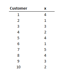
Table 1. Hypothetical data set of 10 customers and their satisfaction rating
A useful way of summarizing data is to determine the center or middle point of scores. Measures of central tendency allow us to determine roughly the center of the scores in the data set. For example, we may measure the satisfaction level (on a scale from 1 to 5) of 10 customers. The data are presented in Table 1. The scores vary considerably, from a low of 1 to a high of 5. We can capture a lot of information about these scores by determining the middle point. By doing so, we get an idea of the value around which the ratings/scores fall. Three statistics that describe the central tendency are the mean, median, and mode.
Mean
The mean is the arithmetic average of all scores in the data set. It is calculated by adding all the scores in the data set and dividing by the total number of observations in the data set. The formula is:

where n = the number of observations in the data set and Σxi is the sum of all scores in the data set. Using the formula, we can calculate the mean of the data in Table 1.

Median
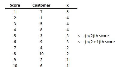
Table 2. Rank order of data from Table 1.
Another measure of central tendency is the median. The median is the middlemost score. In other words, half of the scores have values larger than the median and half have values smaller than the median. If the data set has an odd number of scores, the median is the (n + 1/2)th largest score in the data set. If the data set has an even number of scores, the median is the average of two numbers, the (n/2)th largest score and the (n/2 + 1)th largest score. The first step in calculating the median is to rank order the data from either highest to lowest or lowest to highest. Table 2 provides the rank order of data from Table 1. Since the number of scores in the data set is even, the median is calculated as the average of the two middlemost scores. The median value in the data set is 3.
Mode
The third measure of central tendency is the mode. The mode is the score that occurs most often in the data set. In Table 2, there are two 1s, two 2s, two 3s, three 4s, and one 5. Therefore, the mode of this data set is 4, since it is the most frequently occurring score. It is possible that a data set could have more than one mode. This occurs when two or more values in the data set have the highest frequency.
Variability
While measures of central tendency indicate the middle of the distribution, we also would like to know about the spread of data or how much the data vary around the middle of the distribution. The spread of data is indexed by measures of variability. Measures of variability indicate the extent to which scores are tightly packed together versus spread out. The measures of variability presented here are the variance and the standard deviation. Both measures indicate the spread of data around the mean.
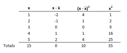 Table 3 contains four columns of numbers. The first column is x, the five score; the second column contains a deviation score from the mean; the third column contains the squared deviation score; and the last column is the squared value of each score.
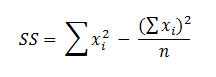
One measure of variability is the variance. Variance, s2, is the sum of the squared deviations about the mean (SS) divided by the number of scores in the data set less one. The formula for the variance is
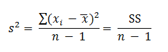
The numerator is the sum of the squared deviations about the mean (SS) and the denominator is called the degrees of freedom. In general, the degrees of freedom for a particular statistic is the number of observations in the data set minus the number of estimated parameters used in the equation. The total number of observations used in the calculation is the sample size (n), and the number of estimated parameters used in the equation is one (the sample mean). It should be noted that some people, in calculating the variance, divide the SS by n instead of n –1. Usually, n is used when the variance is used to describe the present data set, while n – 1 is used to make inferences about the population variance from which the sample is drawn. A more complete discussion between the difference is available in various introductory statistics books. Using the previous equation, the variance of the data is calculated.
The formula for the sum of squared deviations (SS) can be simplified to facilitate hand computation of the variance. The formula for the sum of squares is
Using the data in Table 3, the SS is calculated to be

The value of the variance is 2.5 (10 / 4). You can look at the numerator of the formula to get a sense of what variance tells you about the data. The numerator is the squared deviation of each score from the mean. As the scores are widely spread out from the mean, the numerator increases. Therefore a large variance indicates that the scores are widely spread out, and a small variance indicates that the scores are tightly packed around the mean.
Standard Deviation
Another measure of variability is the standard deviation. The standard deviation is simply the square root of the variance and is denoted by s. The standard deviation for the data in Table 3 is calculated to be s =1.58. The larger the standard deviation, the larger the spread in the data.
If the data are normally distributed, the standard deviation can be used to estimate the percentage of scores that fall within a specified range. By definition, 68 percent of the scores fall within a range whose limits are (mean – 1s) and (mean + 1s), and 95 percent of the scores fall within a range whose limits are (mean – 2s) and (mean + 2s). If the standard deviation is small, a high percentage of the data falls closely around the mean. For our data in Table 3, approximately 68 percent of the data falls within a range from 1.4 to 4.6 (3 – 1.58 to 3+1.58).
Example
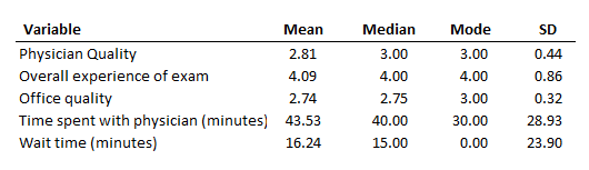
Table 4. Descriptive statistics of items in the patient satisfaction questionnaire
A physician’s office conducted a customer survey to identify their strengths and weaknesses (see Table 4 in previous post on frequencies). In the previous post, we summarized these patient satisfaction ratings using frequencies/percentages. The descriptive statistics (e.g., mean, median, mode and standard deviation) for the patient satisfaction questionnaire are presented here in Table 4.
As we can see from Table 4, the descriptive statistics indicate that customers seem to be satisfied with the overall experience of the exam (ratings can vary from 1 (low) to 5 (high)). Additionally, they seem to be satisfied with the physician quality and overall office quality (ratings can vary from o (low) to 3 (high)).
Although using descriptive statistics to describe the data (mean, median, and mode) summarizes the data even more than using frequencies and percentages, we concluded the same thing about the patients. That is, most of the patients report high levels of quality regarding their patient experience. Also, the wait time indicates that the patients typically had to wait about 15 minutes before seeing the physician. Once in to see the physician, the typical patient spent about 44 minutes with the physician. If we just want to get a general idea of what the satisfaction data tell us, the method of reporting the descriptive statistics is easier than reporting the frequencies.
Summary
This blog included measures of central tendency and measures of variability. Both types of measures summarize information contained in a set of scores. Measures central tendency tell you the middle point of the scores in the data set around which all other scores cluster. Measures of variability determine the extent of spread of the data around the middle point of the distribution.