
As part of my series on Making Sense of Our Big Data World, today’s post is on sampling error. See the overview, Making Sense of Our Big Data World: Statistics for the 99%, to understand the importance and value of understanding statistics and statistical thinking.
This Big Data world is defined by the enormous amount of ever-expanding, diverse data being generated, collected and analyzed by researchers and practitioners alike. While large data sets allow us to gain useful insights about general trends, smaller segments contained within the larger data set are still useful. Consider how the concept of personalization works (e.g., recommendation engines, personlized medicine). From the large data set, we create smaller, homogeneous, data sets to make predictions within smaller groups.
Samples and Populations
Statistically speaking, a population is a “set of entities concerning which statistical inferences are to be drawn.” These inferences are typically based on examining a subset of the population, a sample of observations drawn from that population. For example, if you are interested in understanding the satisfaction of your entire customer base, you measure the satisfaction of only a random sample of the entire population of customers.
Researchers/Scientists rarely, if ever, work with populations when they are studying their phenomenon of interest. Instead, they conduct studies using samples to make generalizations about the population. Specifically, medical researchers rely on the use of a sample of patients to study the effect of a treatment on disease. Polling organizations make nationwide predictions about outcomes of elections based on the responses of only 1000 respondents. Business professionals develop and implement company-wide improvement programs based on the survey results of only a sample of their entire customer base.
Sampling Error
Suppose we have a population of 1,000,000 people and want to make conclusions about their height. We may have only the resources to measure 50 of these people. We use the mean from the sample to estimate the mean of the population.
Based on our sample of 50 randomly selected people, we calculate the mean of their height. Suppose we found the mean height of the sample to equal 62″. Now, let’s place this sample back into the population of 1,000,000 people and take another sample of 50 randomly selected people. Suppose we found the mean of this sample to equal 55″. We notice that there is some difference between the means of the first and second sample of people, both differing from the unknown mean of the population.
For the sake of argument, suppose we knew the mean height of the population to be 60″ with a variance = 50″. The difference of the sample means from population mean is referred to as sampling error. This error is expected to occur and is considered to be random. For the first sample, we happen to select, by chance, people who are slightly taller than the population mean. In the second sample, we selected, again by chance, people who are slightly shorter than the population mean.
Standard Error of the Mean
In the preceding example, we witnessed the effect of sampling error; in one sample the mean was 62″ and in the second sample the mean was 55″. If we did not know the population mean (which is usually the situation), we could not determine the exact amount of error associated with any one given sample. We can, however, determine the degree of error we might expect using a given sample size. We could do so by repeatedly taking a sample of 50 randomly selected people from the population, with replacement, and calculating the mean for each sample. Each mean would be an estimate of the population mean.
If we did this process for 100 different samples, we would have 100 different means (estimates of the population); we could then plot these 100 means to form a histogram or distribution. This distribution of means is itself described by a mean and a standard deviation. This distribution of sample means is called a sampling distribution. The mean of this sampling distribution would be our best estimate of the population mean. The standard deviation of the sampling distribution is called the standard error of the mean (sem). The sem describes the degree of error we would expect in our sample mean. If the population standard deviation is known, we can calculate the sem. The standard error of the mean can be calculated easily using the following formula.
Standard error of the mean = σ /n

Figure 1. Three Distributions. One distribution is based on a sample size of 1 (n = 1). The other two are sampling distributions (n = 10; and n = 100) .
where n is sample size and σ is the population standard deviation (σ²) is the population variance). If we do not know the population standard deviation, we can calculate the standard error of the mean using the sample standard deviation as an estimate of the population standard deviation.
The sampling distributions for two different sample sizes are presented in Figure 1. The population mean (µ) is 60″ and the population variance (σ2) is 50″. The size of sample 1 is 10 and the size of sample 2 is 100. Using the equation above, the standard error of the mean is 2.24″ for sample 1 and .71″ for sample 2. As seen in Figure 1, the degree of sampling error is small when the sample size is large. This figure illustrates the effect of sample size on our confidence in the sample estimate.
When the sample size is 100, we see that any one of our sample means will likely fall close to the population mean (95 percent of the sample means will fall within the range of 58.58″ to 61.42″). When the sample size is 10, our sample means will deviate more from the population mean than do our sample means when using a sample size of 100 (95 percent of the sample means will fall within the range of 53.68″ to 66.32″). In fact, when the sample size equals the population size, the standard error of the mean is 0. That is, when sample size equals population size, the sample mean will always equal the population mean.
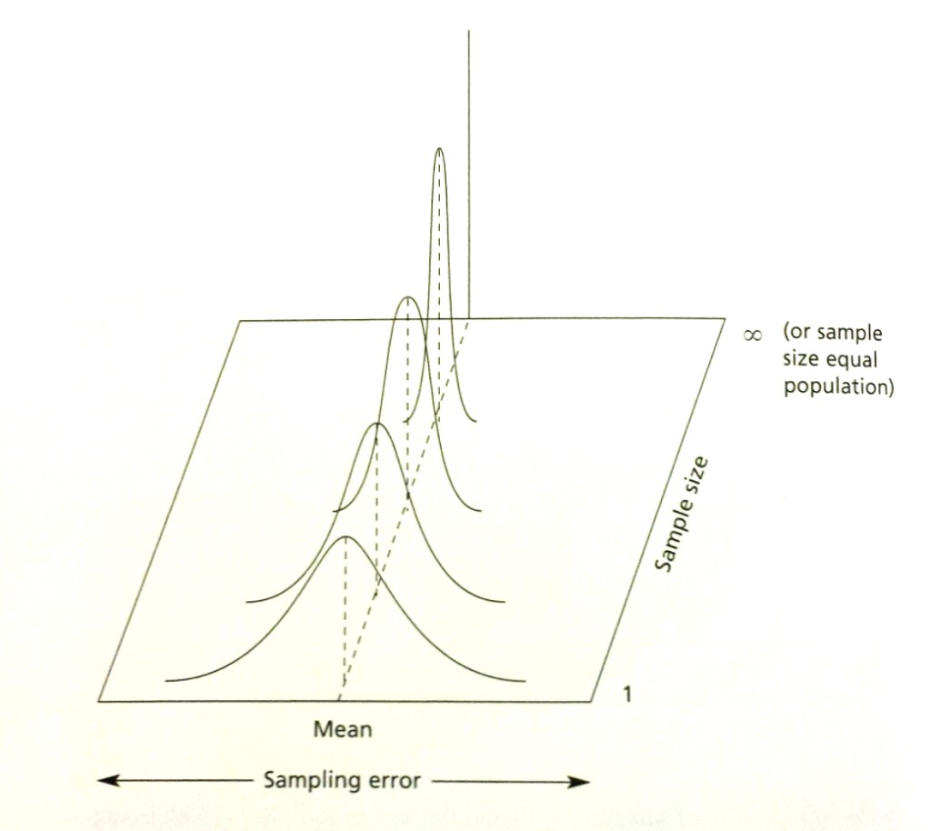
Figure 2. Illustration of the relationship between sample size and sampling error. As sample size increases, sampling error decreases.
Figure 2 illustrates the relationship between sampling error and sample size. As sample size increases, sampling error decreases. When sample size equals one, the standard error of the mean is, by definition, the standard deviation of the population. When sample size equals the size of the population, there is no error in the estimate of the population mean; this sample mean (the sample equals the population) will be exactly the mean of the population. Thus, the standard error of the mean is 0 when sample size equals the size of the population.
Sampling Error and the Need for Inferential Statistics
Inferential statistics is a set of procedures applied to a sample of data in order to make conclusions about the population. Because your sample-based findings are likely different than what you would find using the entire population, applying some statistical rigor to your sample helps you determine if what you see in the sample is what you would see in the population; as such, the generalizations you make about the population need to be tempered using inferential statistics (e.g., regression analysis, analysis of variance).
When Decision-Making Goes Wrong: Tampering with your Business Processes
Used in quality improvement circles, the term, “tampering,” refers to the process of adjusting a business process on the basis of results that are simply expected due to random errors. Putting data interpretation in the hands of people who do not appreciate the notion of sampling error can result in tampering of business processes. As a real example of tampering, I had the experience where an employee created a customer satisfaction trend line covering several quarters. The employee showing me this trend line was implementing operational changes based on the fact that the trend line showed a drop in customer satisfaction in the current quarter. When pressed, the employee told me that each data point on the graph was based on a sample size of five (5!). Applying inferential statistics to the data, I found that the differences across the quarters were not based on real differences, but due, instead, to sampling error. Because of the small sample size, the observed differences across time were essentially noise. Making any changes to the business processes based on these results was simply not warranted.
Big Data Tools will not Create Data Scientists
There has been much talk about how new big data software solutions will help create an army of data scientists to help companies uncover insights in their data. I view these big data software solutions primarily as a way to help people visualize their data. Yes, visualization of your data is important, but, to be of value in helping you make the right decisions for your business, you need to know if the findings you observe in your data are meaningful and real. You can only accomplish this seemingly magical feat of data interpretation by applying inferential statistics to your data.
Simply observing differences between groups is not enough. You need to decipher if the observed differences you see in your metrics (e.g., customer satisfaction, call center) reflects what is happening in the population. Inferential statistics allows you to apply some mathematical rigor to your data that go well beyond merely looking at data and applying the inter-ocular test (aka eyeballing the data). To be of value, data scientists need a solid foundation of inferential statistics and an understanding of sampling error. Only then, can data scientists help their company distinguish signal (e.g., real differences) from the noise (e.g., random error).
Political Polling in National Elections: Example of Sampling Error

Table 1. Summary of polling results from fivethirtyeight.com published on 11/6/2012, one day before the 2012 presidential election. Click image to read entire post.
Nate Silver became a household name when he accurately predicted the winner of the 2008 US presidential election. He used polling data (samples of the population) to help determine who would be the likely winner. When he used the same technique to predict an Obama victory in 2012, he received much criticism from Republicans leading up to election day who said the election was essentially a tossup. As you can see in Table 1, the different polls have slightly different outcomes, some gave Obama a small or larger margin of victory while a few gave Romney the victory. Take a look at the polls within a given state. As you can see, they do not have the same margin of victory for a given candidate. That is because they are based on a sample of likely voters, not the entire population of people who will vote on election day. Because of sampling error, poll results varied across the different polls.
The Power of Aggregation
Let’s compare how Nate Silver and the political pundits made their predictions. While both used publicly available polling data, political pundits appeared to make their predictions based on the results from specific polls. Nate Silver, on the other hand, applied his algorithm to many publicly available polling data at the state level. So, even though the aggregated results of all polls painted a highly probable Obama win, the pundits could still find particular poll results to support their beliefs. (Here is a good summary of pundits who had predicted Romney would win the Electoral College and the popular vote).
No matter your political ideology, I believe that these political polling data (samples) are useful in providing insight about the actual election results (populations), a future event. While Silver’s exact formula for making predictions is unknown, what he does is average many different polling results to make his predictions. His prediction did not say that Obama was certain to win. What it was saying is that if a candidate had a margin of victory as big as Obama had in the polls, he wins 85% of the time. It was not a guarantee that Obama would win. But the odds were in his favor. That is all. Silver’s predictions were not magic. They were simply based on the aggregate of different samples taken from the population.
Summary
Sometimes, opinion and data collide. Some people primarily rely on their personal opinions as a guide to their understanding of the world. Others primarily rely on the use of data as their guide. The prediction of the outcome of US presidential election pits these two views against each other. Based on my examination of recent US political battles, it’s clear that even the use of samples in making predictions is far more accurate than simply using your gut.
Sampling error is the degree to which the sample is different from the population. These differences are a natural part of using only a portion of the population to make conclusions about that population. While we may never know the population (because we can never measure it), we can know how well the values in our sample represent the values from that population. Because the sample will likely be different from the population, it’s important to apply statistical rigor to the sample in order to understand if the sample values paint a real picture of what is going on in the population.


