
When you consider all the machine learning (ML) algorithms, you’ll find there is a subset of very pragmatic ones: neural networks. They usually require no statistical hypothesis and no specific data preparation except for normalization. The power of each network lies in its architecture, its activation functions, its regularization terms, plus a few other features.
When you consider architectures for neural networks, there is a very versatile one that can serve a variety of purposes — two in particular: detection of unknown unexpected events and dimensionality reduction of the input space. This neural network is called autoencoder.
Architecture of the Autoencoder
The autoencoder (or autoassociator) is a multilayer feed-forward neural network, usually trained with the backpropagation algorithm. Any activation function is allowed: sigmoid, ReLU, tanh … the list of possible activation functions for neural units is quite long.
The simplest autoencoder has only three layers: one input layer, one hidden layer and one output layer. More complex structured autoencoders include additional hidden layers. In all autoencoder architectures, though, the number of input units must be the same as the number of output units.
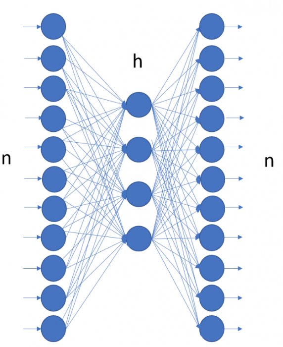
Figure 1. The simplest autoencoder has three layers: one input layer with n units, one hidden layer with h units, and one output layer with n units. Notice the same number n of input and output units.
The autoencoder is usually trained with the backpropagation algorithm — or one of its more modern variations — to reproduce the input vector onto the output layer, hence the same number of input and output neural units. Despite its peculiar architecture, the autoencoder is just a normal feed-forward neural network, trained with the backpropagation algorithm.
Regularization terms and other general parameters, useful to avoid overfitting or to improve the learning process in a neural network, can be applied here as well.
Dimensionality Reduction with the Autoencoder
Let’s consider the autoencoder with a very simple architecture: one input layer with n units, one output layer with also n units, and one hidden layer with h units. If h < n, the autoencoder produces a compression of the input vector onto the hidden layer, reducing its dimensionality from n to h.
In this case, the first part of the network, moving the data from a [1 x n] space to a [1 x h]space plays the role of the encoder. The second part of the network, reconstructing the input vector from a [1 x h] space back into a [1 x n] space, is the decoder. The compression rate is then n/h. The larger the n and the smaller the h, the higher the compression rate.
When using the autoencoder for data compression, the full network is first trained to reproduce the input vector on the output layer. Then, before deployment, it is split in two parts: the encoder (input + hidden layer) and the decoder (hidden + output layer). The two subnetworks are stored separately.
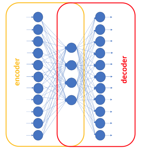
Figure 2. The encoder and the decoder subnetworks in a three-layer autoencoder. The encoder includes the input and hidden layer; the decoder the hidden and output layer.
During the deployment phase, in order to compress an input record, we just pass it through the encoder and save the output of the hidden layer as the compressed record. Then, in order to reconstruct the original vector, we pass the compressed record through the decoder and save the output values of the output layer as the reconstructed vector.
If a more complex structure is used for the autoencoder, i.e., with more than one hidden layer, one of the hidden layers will work as the compressor output, producing the compressed record and separating the encoder from the decoder subnetwork.
Now, the questions when we talk about data compression: How faithfully can the original record be reconstructed? How much information do we lose by using the output of the hidden layer instead of the original data vector? Of course, this all depends on how well the autoencoder performs and on how large our error tolerance is.
During deployment, we apply the network to new data, we denormalize the network output values, and we calculate the chosen error metric — for example, root mean square error (RMSE) — between the original input data and the reconstructed data. The value of the reconstruction error will give us a measure of the quality of the reconstructed data. Of course, the higher the compression rate, the higher the reconstruction error. The problem thus becomes to train the network to achieve an acceptable performance, as per our error tolerance.
Anomaly Detection with the Autoencoder
Another unexpected usage of the autoencoder is to detect the unexpected.
In most classification/prediction problems, we have a set of examples covering all event classes, and based on this data set, we train a model to classify events. However, sometimes the event we want to predict is so rare and unexpected that no (or almost no) examples are available at all. In this case, we do not talk about classification or prediction but about anomaly detection.
An anomaly can be any rare, unexpected, unknown event: a cardiac arrhythmia, a mechanical breakdown, a fraudulent transaction, or other rare, unexpected, unknown event. In this case, since no examples of anomalies are available in the training set, we need to use machine learning algorithms in a more creative way than for conventional, standard classification. The autoencoder structure lends itself to such creative usage, as required for the solution of an anomaly detection problem.
Since no anomaly examples are available, the autoencoder is trained only on non-anomaly examples. Let’s call them examples of the “normal” class. On a training set full of “normal” data, the autoencoder network is trained to reproduce the input feature vector onto the output layer.
The idea is that, when required to reproduce a vector of the “normal” class, the autoencoder is likely to perform a decent job because this is what it was trained to do. However, when required to reproduce an anomaly on the output layer, it will hopefully fail because it won’t have seen this kind of vector throughout the whole training phase. Therefore, if we calculate the distance — any distance — between the original vector and the reproduced vector, we will hopefully see a small distance for input vectors of the “normal” class and a much larger distance for input vectors representing an anomaly.
Thus, by setting a threshold K, we should be able to detect anomalies with the following rule:
xk→”normal” if εk≤K
xk→”anomaly” if εk>K
where εk is the reconstruction error value for input vector xk and K is the set threshold. Such a solution has been already implemented successfully for fraud detection, as described in the blog post “Credit Card Fraud Detection using Autoencoders in Keras – TensorFlow for Hackers (Part VII)” by Venelin Valkov.
In Praise of the Autoencoder
We have shown here two very powerful applications of the neural autoencoder: data compression and anomaly detection.
The beauty of the autoencoder is that, while being so versatile and powerful, it is just a classic feed-forward, backpropagation-trained neural network. It is not a special algorithm and does not need special dedicated software. Any software implementing neural networks will do. The strength and versatility of the autoencoder comes purely from its architecture, where the input vector is reproduced onto the output layer.
Here I have shown two interesting and creative ways of using the neural autoencoder. However, I am sure you can find many more by searching the internet for related scholarly articles or by just activating your imagination and thinking of additional creative tasks for the autoencoder to solve.
As first published in BetaNews.


